Why force uniformity is the figure of merit
A launcher is limited by the peak force its payload can survive, but it is paid in mean force. Every unit of peak-to-mean ratio is capability thrown away. The RopeComb exists to make that ratio small with passive hardware.
Peak / mean force, launch systems compared
System Layout & Operating Principle

The target ratio profile
Impose uniform payload force F, conserve power, and the ratio the transmission must follow falls out as G*(d) = dy/dd:
- d
- the source deceleration (breaking) distance.
- y
- the payload acceleration (launch) distance.
- F
- the force on the payload, uniform by design
- M, m
- source and payload mass
- v0
- speed of the source at the entry of the breaking phase.
- g
- gravity, so 2gd is the work it keeps adding as the source falls
The denominator is the source's remaining speed and the numerator is the payload's: as the source is braked and the payload gains, the required ratio climbs, steeply at the end.
The mechanism
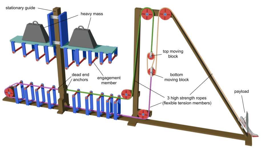
A tension member is reeved alternately over engagement members on a translating carriage and fixed supports, so carriage motion folds it into successive spans. One member of half-width R at depth D contributes
So the ratio rises through the stroke, asymptoting to 2 per member. For an array with offsets si and a fixed second stage k:
Closed form, no integration. Two independent freedoms per member — span width sets how fast a member contributes, offset sets when — and that pair is what lets an arbitrary rising profile be synthesised. Ceiling 2Nk.
Every member is concave; the target is convex
Every member bends the wrong way. The array reaches a convex target only as a chain of concave arcs staggered by their onsets — which is why offsets matter as much as widths, and where the force ripple comes from.
One member, and the staggered sum of several.
Specify the deceleration, not the force
State how hard the source is to be braked, and solve for the force that produces it. Ask for more than the array can reach and the machine gets worse, not merely shorter.
The worked convention is 10 m/s to 4 m/s in 0.100 s, leaving the source 16% of its entry energy over a 0.854 m braking distance, independent of mass ratio. Design force then scales as F ∝ √Mm , and the ideal exit velocity is v0 · √Mm to within a per cent — energy transfer is near total.
4 m/s is a knee, not a derived optimum. Above it the tension member stays loaded throughout; below it traction is lost. Braking to 3.0 m/s buys about 3.3% of exit velocity but carries peak force past the 1.3× bound in every case.
Design by fitting, not by search
Both the array ratio and the target are functions of source displacement, so finding the geometry is a curve fit over 2N parameters:
Plain squared residual — no weighting, no penalties, and no dynamic simulation inside the fit, which is what makes thousands of candidates affordable.
This matters because search does not work. Least squares beats 300,000 random samples by a factor of 7.7 on 150× fewer evaluations, and a structured grid over four intuitive parameters does worse than random sampling: the families a designer would naturally write down do not contain the optimum.
Compliance is required, not a refinement
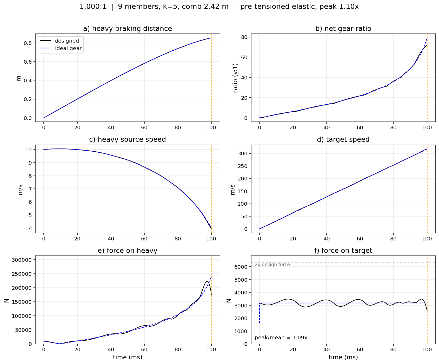
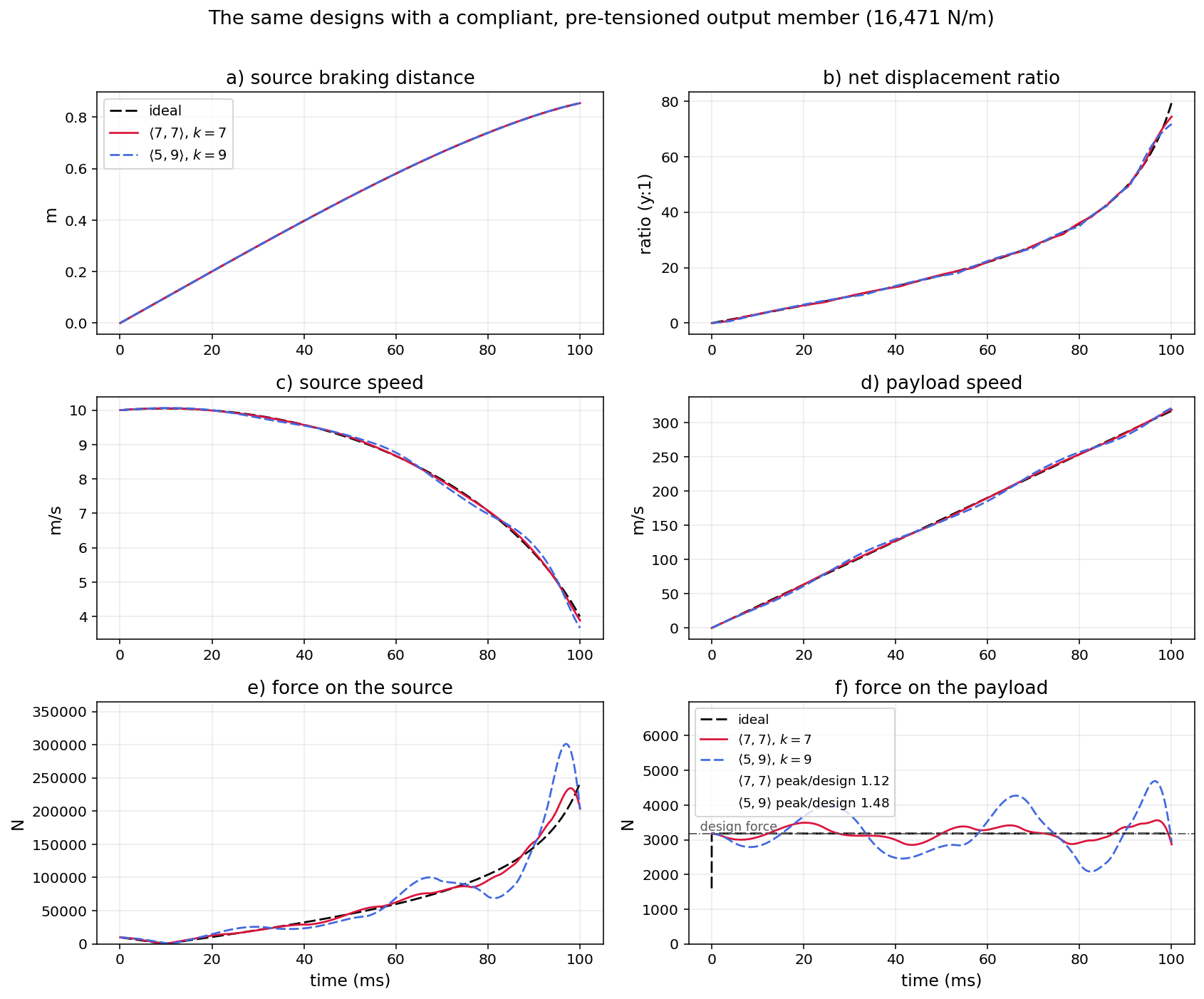
That sawtooth runs at about twice the mean in every canonical design. A compliant, pre-tensioned output member absorbs the transients:
| rigid | compliant | |
| 100:1 | 2.05× | 1.12× |
| 1,000:1 | 2.07× | 1.09× |
| 10,000:1 | 2.10× | 1.19× |
Pre-tension does the work, not compliance alone: started slack, the same apparatus rings at roughly 2.3×. And compliance cannot be engineered away — working strain is of order 1% whatever the fibre.
Severity follows the discreteness of engagement — not the fit residual, and not the mass ratio.
Where the energy goes
Measured against the work needed to raise the source again — through the braking distance as well as the height that set its entry speed — the transmission delivers 86.3% to the payload.
The source mass cancels: efficiency is fixed by entry speed, final speed and braking distance alone, and mass ratio cannot appear. The three simulated designs realise the analytic figure to within 0.4%.
Reality check
The largest omission is the rotational inertia of sheaves in the fast path, which acts exactly as added payload mass and costs a further 9 to 12% of exit velocity — more than any difference between the candidate geometries. Peak-to-mean force is a ratio and survives it; read the velocities as upper bounds.
The models are lossless and no apparatus has been built or measured. Every result here is theoretical or numerical, compared against steam and electromagnetic figures measured on fielded hardware.
The lateral load problem
Cards 09–12 follow doi.org/10.31224/8171.
Everything above hangs off one side of the guide. The carriage reaction — about 23× the source weight, 228 kN at 1,000:1 — is therefore taken at an offset from the guide axis, so the bearings carry an overturning moment while sliding at up to 10 m/s. That friction is dissipation none of the models here count, and it comes straight off exit velocity.
The same geometry costs a second time in the rope. One continuous tension member has to traverse every span of the array and every fall of the fixed stage, paying friction and bending at each element it touches.
The mirror dual array
Split the machine about a central guide and give each half its own tension member, dead-ended on the guide and driving its own moving block at the stage. Two identical arrays cancel the overturning moment by construction, halve the load each array carries, and take ⌊k/2⌋ elements off the busiest rope path — 3 of them at k = 7. They are also identical parts, which halves tooling and spares.
But symmetry does not balance the force. The stage ratio is naturally odd (k = 2p + 1), so the falls cannot be split evenly and the two sides pull unequally by |n1 − n2|/k: 20% at k = 5, 14% at 7, 11% at 9. That is a property of the reeving, not a tolerance — no care in construction reduces it.
Two identical arrays also sum to a net ratio of kG, exactly the single array's, so the payload force profile is unchanged. Mirror symmetry buys the guide and the rope path, and nothing at the payload.
The asymmetric dual array
Nothing requires the halves to match: each rope dead-ends on the guide and drives its own block, so the two sides may draw rope at different rates. In a mirror machine that difference is not just absent but unobservable — identical arrays sum to kG however the falls are split.
Each array pushes on the carriage with its fall count, times its rope’s tension, times its own ratio. Balance is those products meeting:
The array serving more falls takes the smaller ratio — weaken the side doing more work. It also absorbs what symmetry cannot: real ropes run different lengths over different sheave counts, so T1 and T2 are never quite equal.
Order matters too. An engagement steps the slope dG/dd, not the ratio, so the load drifts toward whichever side engaged last, at a rate set by its fall count. Lead with the low-fall array; lead with the other and the residual roughly doubles.
The fit needs one new term:
λ runs continuously from best tracking to exact cancellation — a dial, not a target. And 2N independent members, against a mirror pair’s N, track the target about three times more closely.
What the second array buys
Against a single array, and against a mirror pair, both at the same member count and stage ratio — the second array is hardware you pay for. Seven members per array at k = 7:
| single | mirror | unequal | |
| peak/mean, rigid | 2.44× | 2.44× | 1.93× |
| peak/mean, compliant | 1.40× | 1.40× | 1.12× |
| lateral guide load | 100% | 14.3% | 8.1% |
| elements per rope | 22 | 22 / 22 | 18 / 19 |
The single array has no opposing side, so its whole carriage reaction is an off-axis load: 228 kN of overturning moment on bearings sliding at 10 m/s. A mirror pair cancels that moment — and cancels nothing else. The payload sees the same force, since two identical arrays sum to kG, exactly the single array’s ratio; each rope still runs the full stage; and the residual 14.3% is the odd-k penalty, 1/7 exactly.
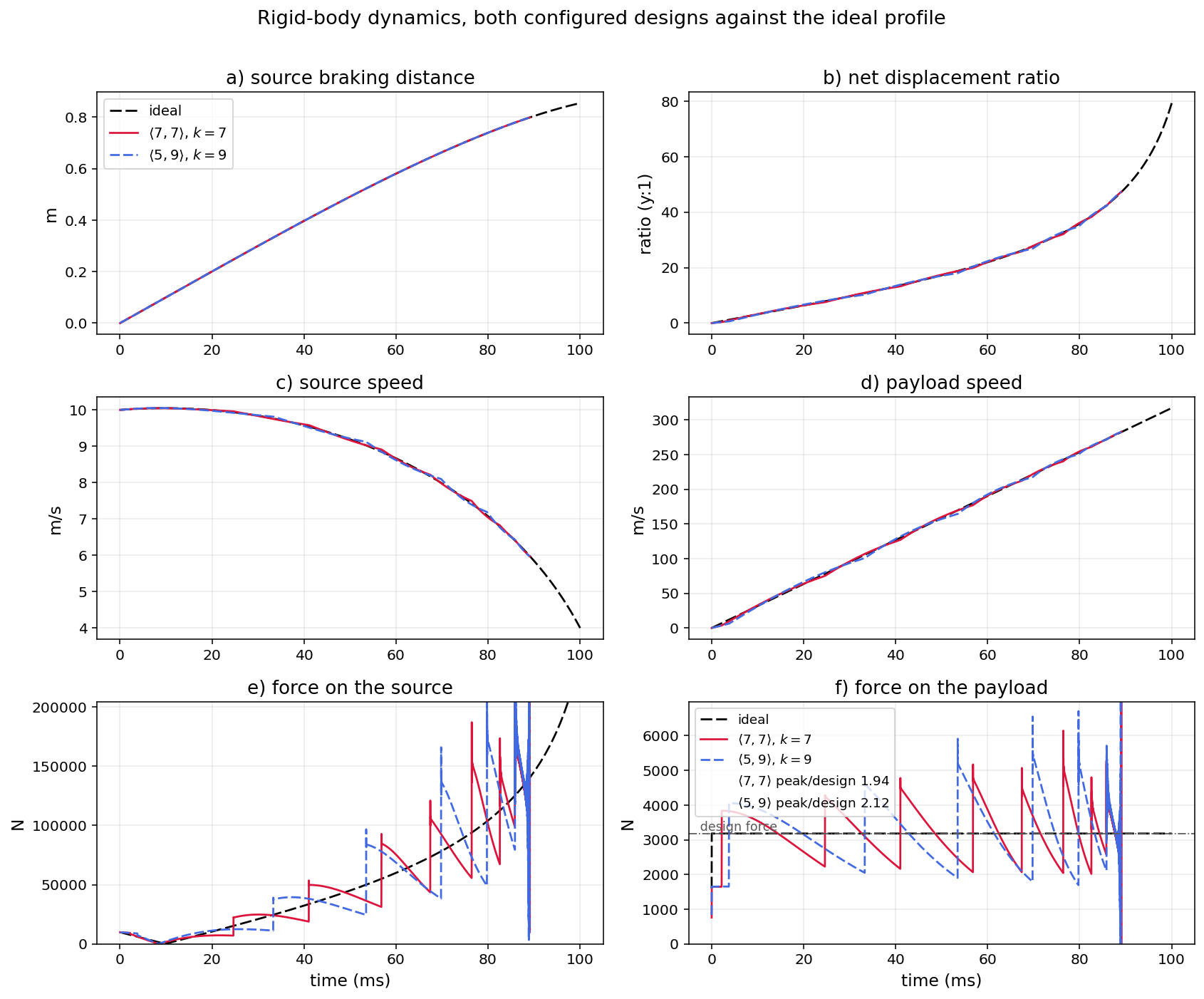
Both remaining columns need the arrays to differ. Anchoring the two ropes separately splits the k falls between them, taking 22 elements to 18 / 19, and the unequal geometry takes the residual to 8.1% — 14.6 kN off bearings carrying 33.7 kN. Five per array at k = 9, from a worse start: 2.88× to 2.11× rigid, 2.19× to 1.48× compliant, 11.1% to 7.0% lateral.
Corresponding spans differ by at most 19 mm at k = 7 and 82 mm at k = 9, against arrays about 2 m wide. The last centimetre does the work.
Exit velocity slips, 321.0 to 318.7 m/s at k = 7: the balance term spends tracking accuracy on cancellation. And the single array is pinned to the dual design’s N and k — like-for-like, not best-against-best.
Simulated; no dual-array machine has been built.
Full treatment, with both configured designs and the derivations, in doi.org/10.31224/8171.
Simulated Dynamics — the 1,000:1 design
The Two Machines, Running
Both loop continuously. Geometry is illustrative and not to scale.
Set your own specification and let the solver search for a comb.
Peak force against array width — every candidate
Score = ((51 - N) / 50) × sqrt(exit_rigid × exit_compliant) / sqrt(0.5 × (peak2mean_rigid² + peak2mean_compliant²))
Mechanism
comb 1:1 · stage and payload rescaled, as labelledForce trace, ratio profile and the full numbers for this run.
Force on payload
Net ratio vs carriage displacement
Peak / mean force, launch systems compared
Run summary
System Geometry
Deceleration & Stroke
Velocity & Performance
What is computed here, and how far to trust it
The geometry is closed form and exact. The dynamics are integrated in the browser by a direct transliteration of the project's Python simulators, including the one-step gear lag, the trapezoidal update and the two-step averaged reaction.
The compliant integrator is verified against the three exported reference runs and reproduces them to the digit: exit velocity within 0.004 m/s, elapsed time within 0.001 ms, peak force within 0.02 N. The target solver returns F = 998.98 / 3169.63 / 10033.82 N against the published 999.0 / 3169.6 / 10033.8.
Peak-to-mean is reported over the first 99.5% of the force trace, the paper's convention: the release is specified to operate before the terminal traction-loss pulse, so that pulse is not experienced by the payload and including it would misstate the load.
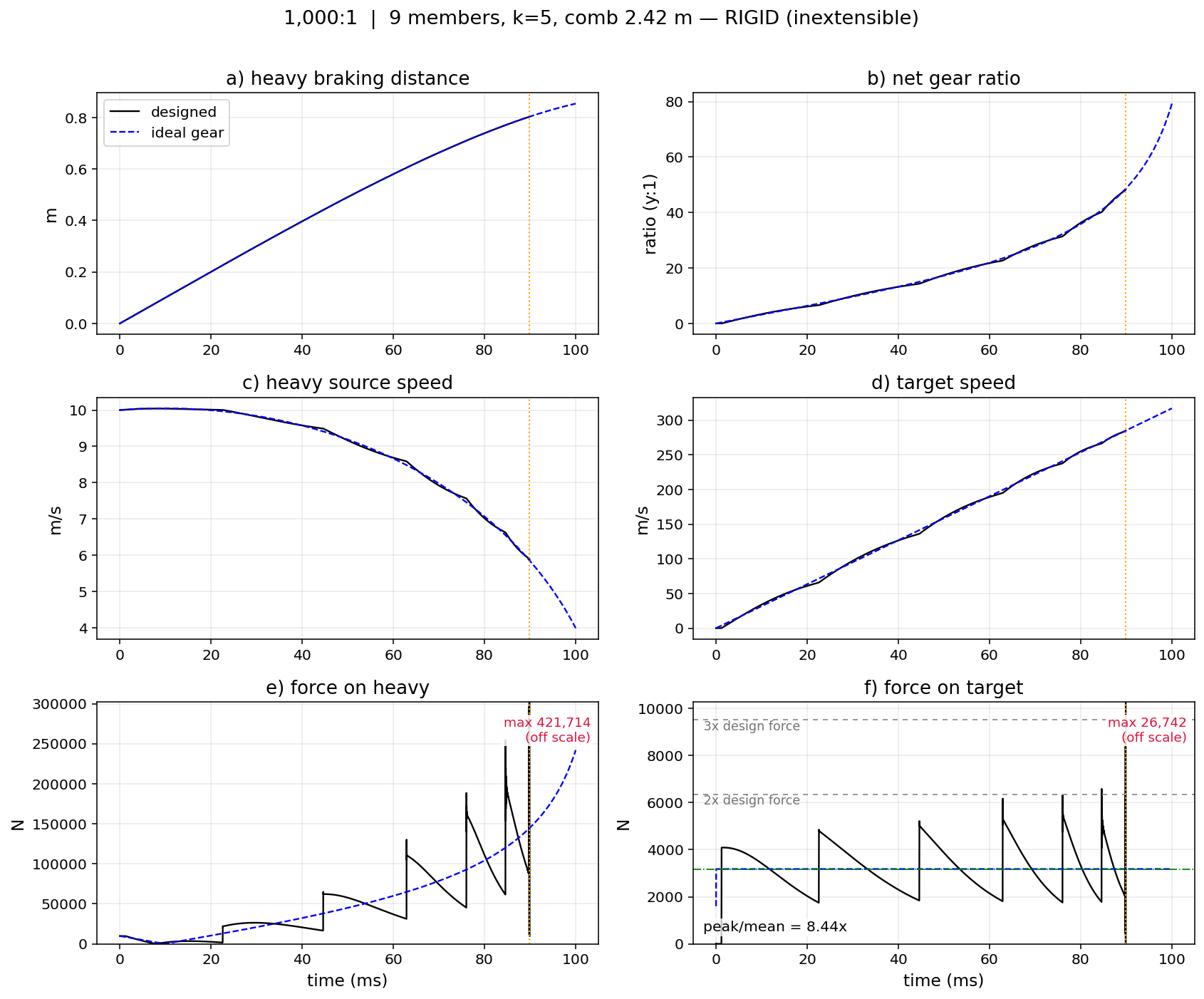
The rigid trace is indicative only. Its termination parameters are not recorded in the reference data, and the run is chaotic in them. This matches the paper's own note that the terminal pulse is the one part of the trace that is not timestep-converged, and that establishing its magnitude would require sub-stepping to the contact transition. Use it to see that an inextensible member diverges, not to read how far.
The geometries shipped on this page predate the paper's joint selection of N and k. They are the earlier hand-selected designs, and their rigid peak-to-mean figures are the superseded 20×/6×/3× family rather than the 2.05×/2.07×/2.10× of the canonical designs. Where this page and the paper disagree, the paper is correct.
Why the solver ranks by simulation, not by fit
The fitting objective matches G, but payload force tracks its slope:
at = G′ vh2 + G ah
So residual predicts force badly. Measured here at 100:1: a fit with rms 0.43 — better than the reference design's 0.48 — produces a peak of 1.50× against the reference 1.24×. Every candidate is therefore simulated and ranked on its actual peak force.
That measurement was made under a target the array could not reach, which is the regime in which the landscape goes multi-modal and the residual stops predicting anything useful. Under a target set by the deceleration rule the landscape is effectively unimodal and restarts agree — within 2.4%, 0.7% and 0.1% on compliant peak-to-mean at 100:1, 1,000:1 and 10,000:1. The return from tuning the objective measures how badly the target is specified; it is a diagnostic, not a design tool. Simulating every candidate remains the safe ranking, but on a well-posed target it mostly breaks ties.
Where restarts do disagree, that spread is shown rather than hidden: it is a property of the problem, not of the solver.
Compliance is a requirement, not a refinement
With an inextensible member the payload outruns the rope tip, the member goes slack, and re-contact arrives as an impulse; successive impulses grow. Severity is governed by the discreteness of engagement — the arc length between successive members relative to the stroke — not by fitting fidelity.
Mass ratio does not order severity. Earlier work, including the reference geometries this page ships, reported severity ordered inversely to mass ratio by a factor of seven. That ordering was an artefact of hand-chosen configurations. Once N and k are selected jointly, the three cases fall within a factor of 1.02 (2.05×, 2.07×, 2.10× rigid) and the sign reverses — the lowest mass ratio is the best behaved rigidly.
Pre-tensioning to the working tension is what matters, not the stiffness value: started slack, the payload mode on that compliance gives roughly 2.3× with the member unloaded for some 11% of the stroke; pre-tensioned, the same apparatus is near 1.03× with no unloaded interval. The result is insensitive to stiffness over the plausible range, and to damping.
Known limits
- Sheave rotational inertia is absent from every model here — the largest single omission, and first-order rather than a correction. Applied post hoc it costs 9 to 12% of exit velocity (neff ≈ 2 to 3 acting as added payload mass). Peak-to-mean force is a ratio and survives it.
- The model is lossless, so energy figures are upper bounds. Friction, member mass and drag are also absent.
- No apparatus has been built or measured. Every figure here is theoretical or numerical, and the steam and electromagnetic figures it is compared against are measured on fielded hardware.
- Above roughly 1000 m/s the rope, not the geometry, becomes the binding constraint: v/c = 0.53 against a UHMWPE critical speed near 1900 m/s, and 0.92 at a safety factor of 3 — past the 0.577c power optimum.
- Minimum practical span is taken as 10 cm. Unconstrained fitting produces 2 cm spans whose slope jumps 2/R are of order 200, and those engage violently.
Algorithmic description of the rigid (inextensible-rope) RopeComb simulation. The carriage motion drives the payload through a rigid unilateral constraint: when the rope is taut, carriage deceleration directly accelerates the payload; if the rope goes slack, the payload enters free flight.
─────────────────────────────────────────────────────────────────────────────
 Algorithm: simulateRigid(M, m, h₀, G(d), dt)
─────────────────────────────────────────────────────────────────────────────
  Inputs
    M       ── source mass  (kg)
    m       ── payload mass (kg)
    h₀      ── source drop height (m); v₀ = √(2·g·h₀)
    G(d)    ── gear-ratio function of source displacement d (m)
    dt      ── time step (s);              default 2×10⁻⁵ s

  Outputs
    time-series of:  t, gear, v_source, v_payload, d_source,
                     d_payload, rope_end, F_source, F_payload, slack

─────────────────────────────────────────────────────────────────────────────

INITIALISE
  v_s    ← √(2·g·h₀)        ── source speed  (m/s)
  v_p    ← 0                 ── payload speed (m/s)
  d_s    ← 0                 ── source displacement (m)
  d_p    ── 0                 ── payload displacement (m)
  G_prev ← 0                 ── gear ratio at previous step
  G_avg  ← 0                 ── average gear over current step
  F_react_prev ← 0          ── reaction force at previous step (N)
  rope_end     ← 0          ── initial rope-end position (m)
  a_p_prev     ← 0          ── payload acceleration at previous step
  a_p    ← 0                 ── payload acceleration (m/s²)
  t      ← 0

LOOP  while  t < t_max  and  a_p < a_max
  t ← t + dt

  ── 1. Update source (heavy) body ─────────────────────────────────────────
  F_net_s    ← M·g  −  G_avg·F_react_prev   ── uses previous-step reaction
  a_s        ← F_net_s / M
  v_s_new    ← v_s + a_s·dt
  d_s_step   ← dt·(v_s_new + v_s) / 2       ── trapezoidal displacement
  d_s        ← d_s + d_s_step
  v_s        ← v_s_new

  ── 2. Update gear ratio ──────────────────────────────────────────────────
  G_new  ← G(d_s)                           ── evaluate comb geometry
  G_avg  ← (G_prev + G_new) / 2
  G_prev ← G_new

  ── 3. Advance rope end (kinematic) ──────────────────────────────────────
  rope_end ← rope_end + d_s_step · G_avg

  ── 4. Update payload body (unilateral rigid constraint) ──────────────────
  free_flight ← (v_p − 0.5·g·dt) · dt       ── free-flight displacement
  taut        ← rope_end − d_p              ── rope-limited displacement

  if free_flight > taut then
    d_p_step ← free_flight                  ── slack: payload is in free flight
    slack    ← true
  else
    d_p_step ← taut                         ── taut: payload constrained by rope
    slack    ← false
  end if

  d_p      ← d_p + d_p_step
  v_p_new  ← 2·(d_p_step / dt) − v_p
  a_p_new  ← (v_p_new − v_p) / dt
  v_p      ← v_p_new
  a_p      ← a_p_new

  ── 5. Compute reaction force ────────────────────────────────────────────
  a1 ← (g + a_p_prev) if a_p_prev > 0 else 0
  a2 ← (g + a_p_new)  if a_p_new > 0 else 0
  F_react_prev ← m · (a1 + a2) / 2

  a_p_prev     ← a_p_new

  ── 6. Record history ─────────────────────────────────────────────────────
  RECORD(t, G_new, v_s, v_p, d_s, d_p, rope_end,
         |F_net_s|, F_react_prev, slack)

END LOOP

RETURN history, peak_force, mean_force, exit_speed, elapsed_time─────────────────────────────────────────────────────────────────────────────
Algorithm: G(d) ─ instantaneous gear ratio of the comb at displacement d
─────────────────────────────────────────────────────────────────────────────
Inputs
R[1..N] ── half-widths of the N sheaves / buckets (m)
s[1..N] ── axial offsets of the N pins (m)
k ── number of rope wraps (stage count)
d ── current source displacement (m)
Output: total gear ratio G (dimensionless)
─────────────────────────────────────────────────────────────────────────────
FUNCTION G(d):
total ← 0
for i ← 1 to N do
D ← d − s[i] depth into sheave i
if D > 0 then
total ← total + 2·D / √(R[i]² + D²)
end for
return k · totalThe full Python reference implementation for the RopeComb simulation, fitting solver, and canonical cases has been packaged and published as an open-source library.
Python Reference Implementation
View the full repository, solvers, and simulation code on GitHub.